how to add line of best fit in excel

Note:These steps apply to Office 2013 and newer versions. Looking for Office 2010 steps?

Add a trendline

Your browser does not support video.

Select a chart.
Select the + to the top right of the chart.
Select Trendline.

Note:Excel displays the Trendline option only if you select a chart that has more than one data series without selecting a data series.
In the Add Trendline dialog box, select any data series options you want, and click OK.

Format a trendline

Click anywhere in the chart.
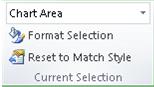
On the Format tab, in the Current Selection group, select the trendline option in the dropdown list.
Click Format Selection.
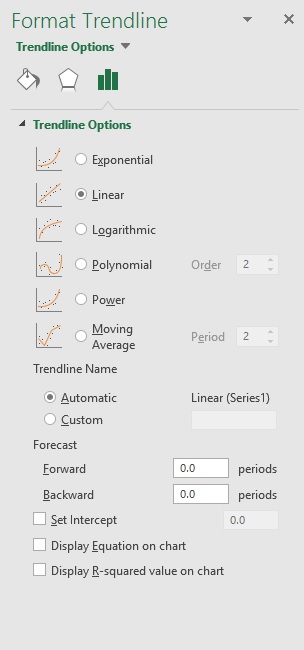
In the Format Trendline pane, select a Trendline Option to choose the trendline you want for your chart. Formatting a trendline is a statistical way to measure data:
Set a value in the Forward and Backward fields to project your data into the future.

Add a moving average line

You can format your trendline to a moving average line.

Click anywhere in the chart.
On the Format tab, in the Current Selection group, select the trendline option in the dropdown list.
Click Format Selection.
In the Format Trendline pane, under Trendline Options, select Moving Average. Specify the points if necessary.

Note:The number of points in a moving average trendline equals the total number of points in the series less the number that you specify for the period.

Add a trend or moving average line to a chart in Office 2010

On an unstacked, 2-D, area, bar, column, line, stock, xy (scatter), or bubble chart, click the data series to which you want to add a trendline or moving average, or do the following to select the data series from a list of chart elements:
1. Click anywhere in the chart.
  
  This displays the Chart Tools, adding the Design, Layout, and Format tabs.
2. On the Format tab, in the Current Selection group, click the arrow next to the Chart Elements box, and then click the chart element that you want.
Note:If you select a chart that has more than one data series without selecting a data series, Excel displays the Add Trendline dialog box. In the list box, click the data series that you want, and then click OK.
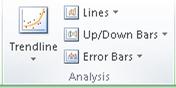
On the Layout tab, in the Analysis group, click Trendline.

Do one of the following:

Click a predefined trendline option that you want to use.

Note:This applies a trendline without enabling you to select specific options.
Click More Trendline Options, and then in the Trendline Options category, under Trend/Regression Type, click the type of trendline that you want to use.

Use this type	To create
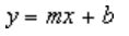
Linear	A linear trendline by using the following equation to calculate the least squares fit for a line: where m is the slope and b is the intercept.
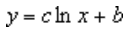
Logarithmic	A logarithmic trendline by using the following equation to calculate the least squares fit through points: where c and b are constants, and ln is the natural logarithm function.
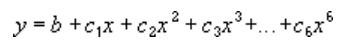
Polynomial	A polynomial or curvilinear trendline by using the following equation to calculate the least squares fit through points: where b and are constants.
Power	A power trendline by using the following equation to calculate the least squares fit through points: where c and b are constants. Note:This option is not available when your data includes negative or zero values.
Exponential	An exponential trendline by using the following equation to calculate the least squares fit through points: where c and b are constants, and e is the base of the natural logarithm. Note:This option is not available when your data includes negative or zero values.
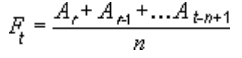
Moving average	A moving average trendline by using the following equation: Note:The number of points in a moving average trendline equals the total number of points in the series less the number that you specify for the period.
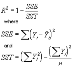
R-squared value	A trendline that displays an R-squared value on a chart by using the following equation: This trendline option is available on the Options tab of the Add Trendline or Format Trendline dialog box. Note:The R-squared value that you can display with a trendline is not an adjusted R-squared value. For logarithmic, power, and exponential trendlines, Excel uses a transformed regression model.

If you select Polynomial, type the highest power for the independent variable in the Order box.
If you select Moving Average, type the number of periods that you want to use to calculate the moving average in the Period box.
If you add a moving average to an xy (scatter) chart, the moving average is based on the order of the x values plotted in the chart. To get the result that you want, you might have to sort the x values before you add a moving average.
If you add a trendline to a line, column, area, or bar chart, the trendline is calculated based on the assumption that the x values are 1, 2, 3, 4, 5, 6, etc.. This assumption is made whether the x-values are numeric or text. To base a trendline on numeric x values, you should use an xy (scatter) chart.
Excel automatically assigns a name to the trendline, but you can change it. In the Format Trendline dialog box, in the Trendline Options category, under Trendline Name, click Custom, and then type a name in the Custom box.

Tips:

You can also create a moving average, which smoothes out fluctuations in data and shows the pattern or trend more clearly.
If you change a chart or data series so that it can no longer support the associated trendline — for example, by changing the chart type to a 3-D chart or by changing the view of a PivotChart report or associated PivotTable report — the trendline no longer appears on the chart.
For line data without a chart, you can use AutoFill or one of the statistical functions, such as GROWTH() or TREND(), to create data for best-fit linear or exponential lines.

On an unstacked, 2-D, area, bar, column, line, stock, xy (scatter), or bubble chart, click the trendline that you want to change, or do the following to select it from a list of chart elements.
1. Click anywhere in the chart.
  
  This displays the Chart Tools, adding the Design, Layout, and Format tabs.
2. On the Format tab, in the Current Selection group, click the arrow next to the Chart Elements box, and then click the chart element that you want.
On the Layout tab, in the Analysis group, click Trendline, and then click More Trendline Options.
To change the color, style, or shadow options of the trendline, click the Line Color, Line Style, or Shadow category, and then select the options that you want.

On an unstacked, 2-D, area, bar, column, line, stock, xy (scatter), or bubble chart, click the trendline that you want to change, or do the following to select it from a list of chart elements.
1. Click anywhere in the chart.
  
  This displays the Chart Tools, adding the Design, Layout, and Format tabs.
2. On the Format tab, in the Current Selection group, click the arrow next to the Chart Elements box, and then click the chart element that you want.
On the Layout tab, in the Analysis group, click Trendline, and then click More Trendline Options.
To specify the number of periods that you want to include in a forecast, under Forecast, click a number in the Forward periods or Backward periods box.

On an unstacked, 2-D, area, bar, column, line, stock, xy (scatter), or bubble chart, click the trendline that you want to change, or do the following to select it from a list of chart elements.
1. Click anywhere in the chart.
  
  This displays the Chart Tools, adding the Design, Layout, and Format tabs.
2. On the Format tab, in the Current Selection group, click the arrow next to the Chart Elements box, and then click the chart element that you want.
On the Layout tab, in the Analysis group, click Trendline, and then click More Trendline Options.
Select the Set Intercept = check box, and then in the Set Intercept = box, type the value to specify the point on the vertical (value) axis where the trendline crosses the axis.

Note:You can do this only when you use an exponential, linear, or polynomial trendline.

On an unstacked, 2-D, area, bar, column, line, stock, xy (scatter), or bubble chart, click the trendline that you want to change, or do the following to select it from a list of chart elements.
1. Click anywhere in the chart.
  
  This displays the Chart Tools, adding the Design, Layout, and Format tabs.
2. On the Format tab, in the Current Selection group, click the arrow next to the Chart Elements box, and then click the chart element that you want.
On the Layout tab, in the Analysis group, click Trendline, and then click More Trendline Options.
To display the trendline equation on the chart, select the Display Equation on chart check box.

Note:You cannot display trendline equations for a moving average.

Tip:The trendline equation is rounded to make it more readable. However, you can change the number of digits for a selected trendline label in the Decimal places box on the Number tab of the Format Trendline Label dialog box. (Format tab, Current Selection group, Format Selection button).

On an unstacked, 2-D, area, bar, column, line, stock, xy (scatter), or bubble chart, click the trendline for which you want to display the R-squared value, or do the following to select the trendline from a list of chart elements:
1. Click anywhere in the chart.
  
  This displays the Chart Tools, adding the Design, Layout, and Format tabs.
2. On the Format tab, in the Current Selection group, click the arrow next to the Chart Elements box, and then click the chart element that you want.
On the Layout tab, in the Analysis group, click Trendline, and then click More Trendline Options.
On the Trendline Options tab, select Display R-squared value on chart.

Note:You cannot display an R-squared value for a moving average.

On an unstacked, 2-D, area, bar, column, line, stock, xy (scatter), or bubble chart, click the trendline that you want to remove, or do the following to select the trendline from a list of chart elements:
1. Click anywhere in the chart.
  
  This displays the Chart Tools, adding the Design, Layout, and Format tabs.
2. On the Format tab, in the Current Selection group, click the arrow next to the Chart Elements box, and then click the chart element that you want.
Do one of the following:
1. On the Layout tab, in the Analysis group, click Trendline, and then click None.
2. Press DELETE.

Tip:You can also remove a trendline immediately after you add it to the chart by clicking Undo Undo button on the Quick Access Toolbar, or by pressing CTRL+Z.